Andy Jiménez
Financial Data Scientist
Bachelor's Degree in Finance.
Programming projects in Finance fields such as Financial Modelling, Stock Prediction, Portfolio Optimization, Valuation, Forecasting Time-series, etc.
View My LinkedIn Profile
Home
Forecasting Google Searches
Click Here to see Code
Project Description: The objective of this project is to forecast google trends data appying time-series tools in Python.
We will be using statsmodels libraries to achieve this goal.
Get data from Google Trends
As an example, we will use “pajamas” and “bikinis” worldwide Google searches. You can get this data directly from Google Trends.
Plot series:
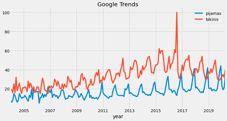
Observe how these series complements one each other. While people search “pajamas” in google, searches for “bikinis” are no longer popular, and viceversa. There is a seasonal component, obviously.
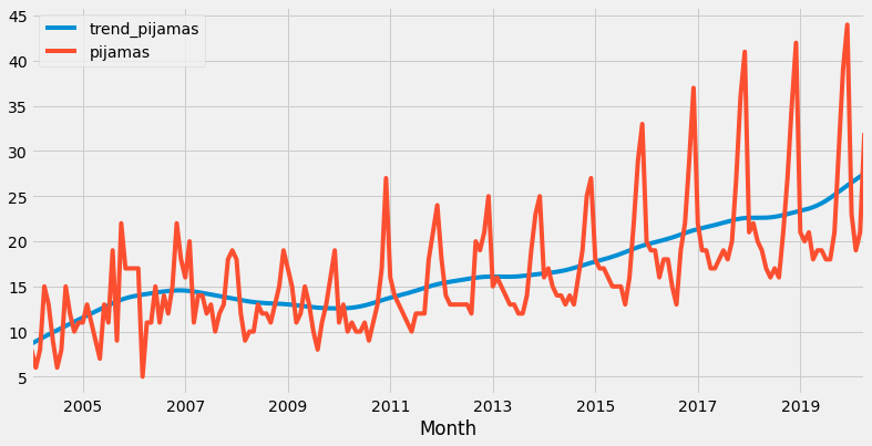
Trend
Statsmodel library can easily get the trending for “pajamas” series.
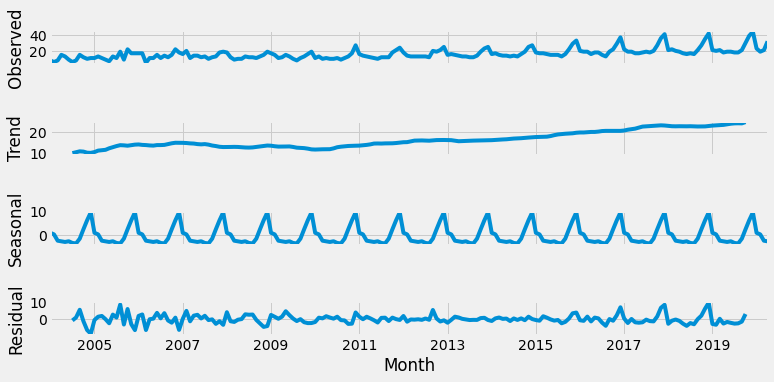
And if we want decompose the time-series, this library plot a nice graph with Trend, Seasonal and Residuals components of the serie.
Look at stationarity
Stationarity is a statistical assumption that a time-series has:
-
Constant mean
-
Constant variance
-
Autocovariance does not depend on time
Clearly, the pajamas time-serie doesn’t have a constant mean over time.
Testing for Stationarity
We can use the Augmented Dickey-Fuller unit root test.
An augmented Dickey–Fuller test (ADF) tests the null hypothesis that a unit root is present in a time series sample.
Basically, we are trying to whether to accept the Null Hypothesis H0 (that the time series has a unit root, indicating it is non-stationary) or reject H0 and go with the Alternative Hypothesis (that the time series has no unit root and is stationary).
We end up deciding this based on the p-value return.
A small p-value (typically ≤ 0.05) indicates strong evidence against the null hypothesis, so you reject the null hypothesis.
A large p-value (> 0.05) indicates weak evidence against the null hypothesis, so you fail to reject the null hypothesis.
Run the ADF Test
Augmented Dickey-Fuller Test:
ADF Test Statistic : 0.8444347153424413
p-value : 0.9923206019227581
#Lags Used : 13
Number of Observations Used : 182
weak evidence against null hypothesis, time series has a unit root, indicating it is non-stationary
Correct Stationary
There are two major reasons behind non-stationarity of a time-series:
-
Trend – varying mean over time.
-
Seasonality – variations at specific time-frames.
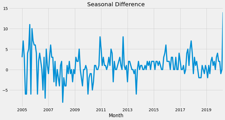
Differencing
One of the most common methods of dealing with both trend and seasonality is differencing. In this technique, we take the difference of the observation at a particular instant with that at the previous instant. This mostly works well in improving stationarity.
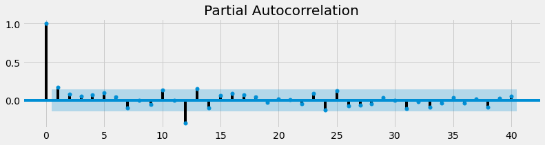
Autocorrelation and Partial Autocorrelation
An autocorrelation plot shows the correlation of the series with itself, lagged by x time units.
How do we determine p, d, and q? For p and q, we can use ACF and PACF plots (below).
Autocorrelation Function (ACF): Correlation between the time series with a lagged version of itself.
Partial Autocorrelation Function (PACF): Measures the correlation between the time-series with a lagged version of itself but after eliminating the variations already explained by the intervening comparisons.
Plot Autocorrelation plots:
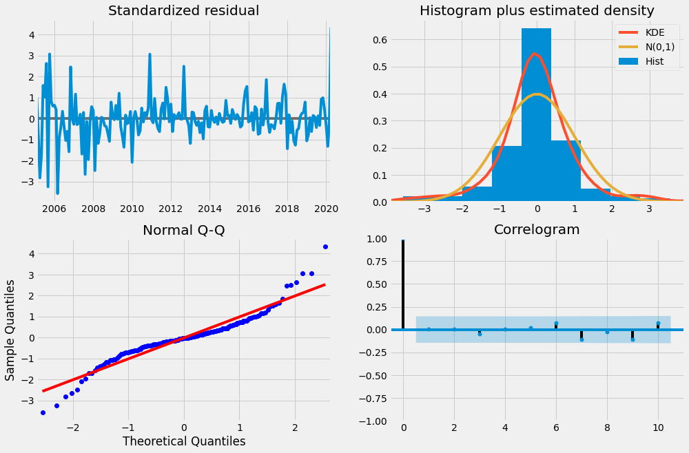
Seasonal ARIMA model
Finally we can use our Seasonal ARIMA model now that we have an understanding of our data:
Residuals are useful in checking whether a model has adequately captured the information in the data. Residual must be uncorrelated and zero mean.
Plot the Residual Diagnostics.
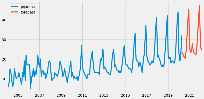
Prediction of Future Values