Financial Analysis and Markowitz’s Efficient Frontier for Colombian Stocks

Click Here to see Code

Project description: Financial analysis for colombian stocks and portfolio optimization methods (Monte Carlo approach and Scipy’s “optimize” function for minimizing or maximizing objective functions subject to constraints).

This Project uses the API provided by Investpy to get historical data for colombian stocks.

The historical data for U.S. stocks can easily get from Yahoo Finance.

Historical Data

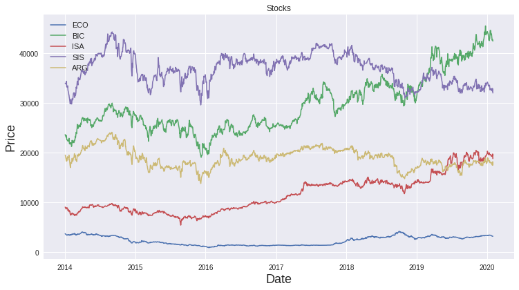
For the purpose of this project we will get the historical prices from Ecopetrol (ECO), Bancolombia (BIC), Interconnection Electric (ISA), Grupo de Inversiones Suramericana (SIS) and Grupo Argos (ARG). We set a history range from ‘01/01/2014’ to ‘01/02/2020’ (‘%d/%m/%Y’).

Note: Investpy just let us get the historical price for one stock at a time, so we need to iterate over the ticker list and concatenate dataframes for each stock. The result will be a one dataframe containing the daily close price for each ticker.

Date	ECO	BIC	ISA	SIS	ARG
2020-01-31	3180.0	42440.0	18800.0	32000.0	17480.0

Plotting useful information

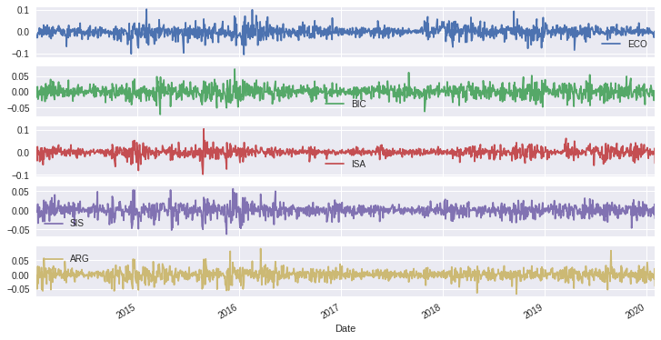
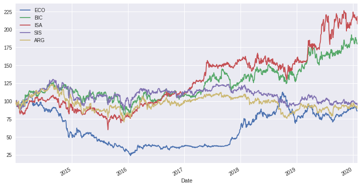
With a few lines of code in Python, we can easily plot the stocks prices, the log mean return and the cumulative return over time.

Cumulative return shows us that if we were invested 1 monetary unit in ISA in 2014, at the end of the analyzed period, we would get almost 225 monetary units (fee free).

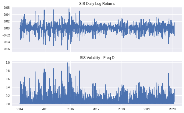
We can plot the daily returns for ISA and below plot its daily realized volatility.

The formula for realized volatility is as follows:

$\Large RV \equiv \sqrt{\sum_{i=1}^{T} r_t^2}$

Where $\Large r_t =$ return at period t

The grahp shows us that the maximum daily volatility for ISA is $\Large sigma \approx 1$

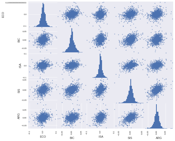
Log Return Distributions and Correlation Matrix

Pandas provides us an easy way to plot a scatter matrix with the distribution of returns for each stock and the correlation between them.

Selecting two stock we can run an OSL (ordinary least-squares) analysis and then examine the correlation for a fixed window over time (Window period = 252 days).

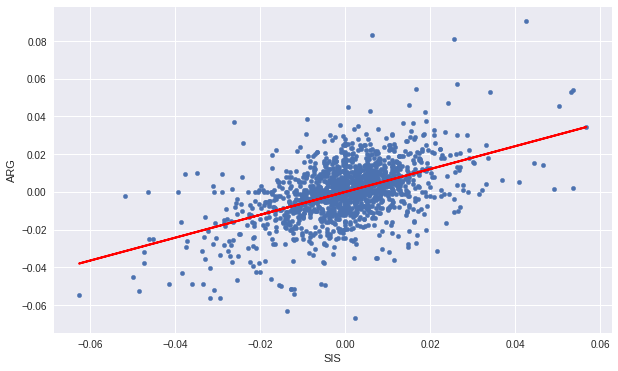
The graph shows postive corretation over time between the two stocks:

Statistics and Normality Tests

Next graph shows the QQ plot for ECO. Clearly, the sample quantile values do not lie on a straight line, indicating “non-normality.” On the left and right sides there are many values that lie well below the line and well above the line, respectively. In other words, the time series data exhibits fat tails.

We can run a few statistics to validate the hypothesis that the sample data are normally distributed.

Results for symbol ECO	Value
Skew of data set	-0.097
Skew test p-value	0.126
Kurt of data set	3.276
Kurt test p-value	0.000
Norm test p-value	0.000

The p -values of the kurtosis and nomal tests are zero, rejecting the test hypothesis. We might have to use richer models that are able to generate fat tails (e.g., models with stochastic volatility or jump diffusion models).

Opmitization Methods

Monte Carlo Approach: Optimal Portfolio

With this method we will try to discover the optimal weights by simply creating a large number of random portfolios, and extract within all these randomly portfolios the one who has the maximum sharpe Ratio (Optimal Portfolio) and in the other hand, the one who has the minimun variance (Minimun Variance Portfolio). For sharpe ratio calculations we set a risk free = 0.

Before to do that, we will review some formulas:

Portfolio Standard Deviation

$\Large \sigma_{port} = \sqrt{\sum_{i=1}^{n}w_i^2\sigma_i^2 + \sum_{i=1}^{n}\sum_{i=1}^{n}w_iw_jCov_{ij}}$

wehere:

$\Large \w_{i} =$ the weights of individual assets in the portfolio, where weights are determined by the proportion of value in the portfolio

$\Large \sigma_i^2 =$ the variance of rates of return for asset i

$\Large \Cov_{ij} =$ the variance of rates of return for asset i, where $\large \Cov_{ij} = r_{ij}\sigma_i\sigma_j$

Portfolio Expected Return

$\Large \bar{R}_{port} = \sum_{i=1}^{n}w_ir_i$

where:

$\Large \w_{i} =$ the proportion, or weights of total funds invested in security i

$r_i =$ expected return for security i

Sharpe Ratio

$\Large SR = \frac{\bar{R}_{port} - Rf}{\sigma_{port}}$

where:

$Rf =$ Riskfree rate

With Numpy library we can simple generate 100k randomly portfolio combinations. The results will store in a Python dict:

dict_keys(['Returns', 'Volatility', 'Sharpe Ratio', 'ECO Weight', 'BIC Weight', 'ISA Weight', 'SIS Weight', 'ARG Weight'])

Then plot the results:

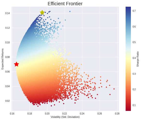
The red star is the portfolio with the minimum variance. Here the portfolio composition:

Return	0.069986
Volatility	0.164826
Sharpe Ratio	0.424605
ECO Weight	0.078844
BIC Weight	0.240285
ISA Weight	0.204278
SIS Weight	0.348250
ARG Weight	0.128342

The yellow star is the portfolio with the maximum sharpe ratio. Here the portfolio composition:

Return	0.140984
Volatility	0.194283
Sharpe Ratio	0.725665
ECO Weight	0.020040
BIC Weight	0.410700
ISA Weight	0.561843
SIS Weight	0.006014
ARG Weight	0.001402

Linear Programming with Scipy: Optimal Portfolio

Using Scipy we quick resolve the optimiaztion problem by minimizing functions. We will be using the ‘SLSQP’ method in our “minimize” function (which stands for Sequential Least Squares Programming, and the “eq” argument means we are looking for our function to equate to zero, otherwise speaking, weights of portfolio must sum to 1 (no short positions).

The “bounds” specify that each individual stock weight must be between 0 and 1.

Minimization variance portfolio function

To find the weights for Minimum Variance Portfolio we must to run this piece of code to minimize the objective function:

def min_func_variance(weights):
    return statistics(weights)[1]

cons = ({'type': 'eq', 'fun': lambda x:  np.sum(x) - 1}) # No Short positions

bnds = tuple((0, 1) for x in range(num_stocks))
    
optv = sco.minimize(min_func_variance, equal_weights, method='SLSQP',
                       bounds=bnds, constraints=cons)

Here the optimal weights:

ECO	BIC	ISA	SIS	ARG
0.09	0.24	0.19	0.34	0.14

# [Portfolio Return, Portfolio Std, Sharpe Ratio]

array([0.06907, 0.16479, 0.41915])

Maximizing sharpe ratio function

Scipy offers a “minimize” function, but no “maximize” function, so maximization of the Sharpe ratio is analogous to the minimisation of the negative Sharpe ratio:

def min_func_sharpe(weights):
    return -statistics(weights)[2]
    
cons = ({'type': 'eq', 'fun': lambda x:  np.sum(x) - 1}) # No Short positions

bnds = tuple((0, 1) for x in range(num_stocks))

opts = sco.minimize(min_func_sharpe, equal_weights, method='SLSQP',
                       bounds=bnds, constraints=cons)

Here the optimal weights (for sharpe ratio calculations we set a risk free = 0):

ECO	BIC	ISA	SIS	ARG
0.0	0.4454	0.5546	0.0	0.0

# [Portfolio Return, Portfolio Std, Sharpe Ratio]

array([0.1437 , 0.196  , 0.73318])

You’ll notice that the composition and metrics of both portfolios is similar to portfolios found through the Monte Carlo method. We will always experience some discrepancies between them. In fact, we can run enough simulated portfolios to replicate the exact weights, but never they would be the exact weights for optimal portfolio.

Finally, we plot the efficient boundary with optimal weights for each portfolio:

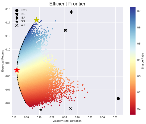
Obviously, if we were invested 100 percent in ISA, the return would be higher but the risk would be too.

PyPortfolioOpt Library

Without doubt, this is the easiest way to find the optimal weights for a given portfolio. With a few lines of code this library is able to optimize a portfolio in seconds, and tell us how many shares we can buy at the lastest close price of the stock.

Optimal Weights

{'ECO': 0.0, 'BIC': 0.43204, 'ISA': 0.56796, 'SIS': 0.0, 'ARG': 0.0} 

Expected annual return: 14.4%
Annual volatility: 19.7%
Sharpe Ratio: 0.73
(0.14406456150209906, 0.19653202475586729, 0.7330335179778285)

If we want invest $10 million COP in this Optimal portfolio, we should buy 102 shares of BIC and 301 shares of ISA, and expect an annual return of 14.4% (Markowitz’s Modern Portfolio Theory).

Discrete Allocation: {'BIC': 102.0, 'ISA': 301.0}
Funds Remaining: $12320.00