Neural Networks to Predict Stock Price

Click Here to see Code

Proeject Description: Employing neural networks to approach financial time series and making predictions of the price movements. Using LSTM to predict stock prices can actually produce impressive results compared to other, more than traditional statistical methods of technical analysis.

We will be using Ecopetrol Stock as an example. You can get the stock price data installing Investpy library.

Long Short Term Memory

One special type of neural networks is a Long Short-Term Memory (LSTM), an artificial Recurrent Neural Network (RNN) architecture extremely powerful for time series modelling. In a simple way, LSTM predictions are always conditioned by the past experience of the network’s inputs.

Let’s see. Humans don’t start their thinking from scratch every second. You understand each word based on your understanding of previous words. Your thoughts have persistence. RNN are networks with loops in them, allowing information to persist.

But there’s a problem with RRN. In practice, they don’t seem to be able to learn from ‘long-term dependencies”. Thankfully, LSTMs don’t have this problem. Remembering information for long periods of time is practically their default behavior.

Ok, let’s dive in to check it!!

 

Get Data

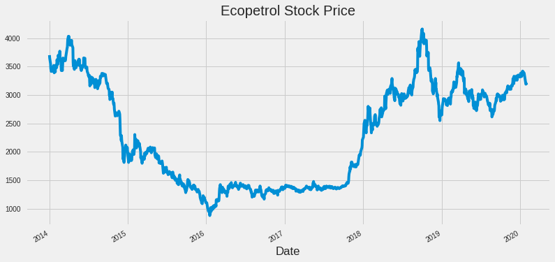
Before to run the LSTM model, we will take a look at the time-serie and calculate its drawdown over time.

 

Drawdown Analysis

The Drawdown is defined as the worst return we would experience if we buy at very highest peak and sell at very lowest point. It measures potential losses, and therefore it is a downside risk measure.

First calculate the max peaks:

 

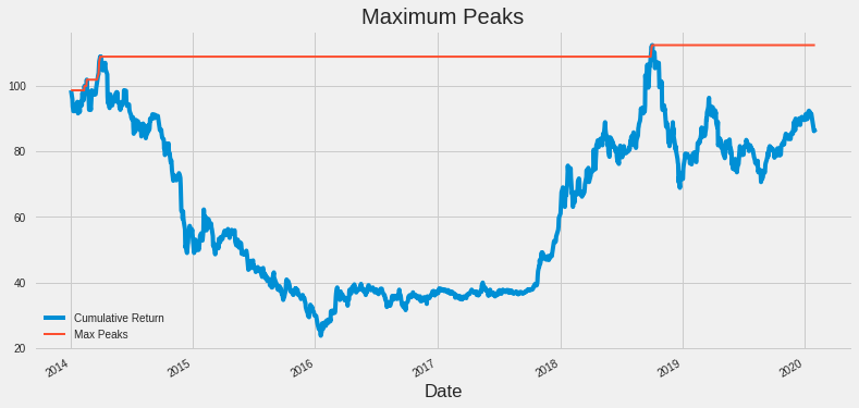
Then, plot the percentage of losses. In this case there’s a huge loose within 2014 and 2016. In 2016 reaches the max drawdown:

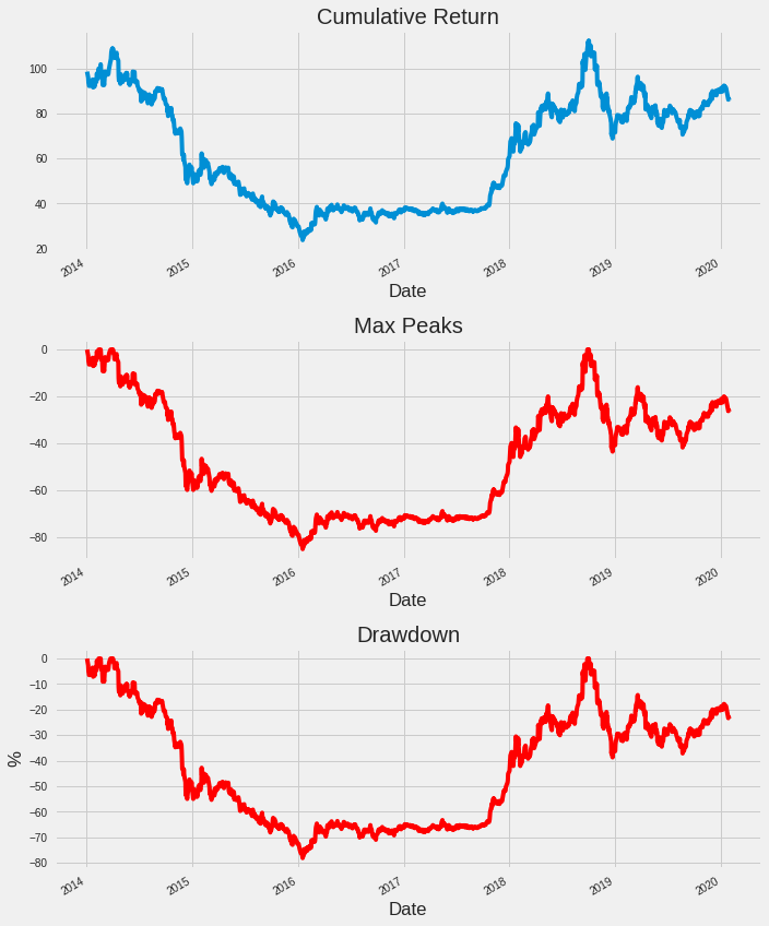
Max drawdown: -78.0%
Date max drawdown: 2016-01-18 00:00:00

 

LSTM Model in Practice

In this section, there are two parts: In the first part (Model 1), we will set the parameters taking a higher number of neurons and epochs. In the second, we will reduce these numbers and compare the results. In both sections, we will use the Adam method which is a method for Stochastic Optimization.

The model uses historical data from the past 6 years. To train the model, 80% of this data will be used, i.e. daily closing prices. At the end, we will check how well would the model have predicted the stock price for the last 90 days, and finally, we will predict the next day close price and compare it to real close price.

 

Model 1

First, we have to normalize the close prices:

data = df.filter(['Close']).copy()
min_max_scaler = preprocessing.MinMaxScaler()
data['Close'] = min_max_scaler.fit_transform(data['Close'].values.reshape(-1,1))

Then, reshape data to obtain a 3D array:

scale_df.shape
(1391, 91, 1)

Set the parameters for the model and run it. It may take a few minutes running depending the number of epochs we set:

neurons = [256, 256, 32, 1]
shape = [90, 1, 1] 
dropout = 0.2 
decay = 0.5
epochs = 100

Once we train the model, we’ll calculate its MSE. For this model we got a MSE ~ 0.002105. Not bad at all.

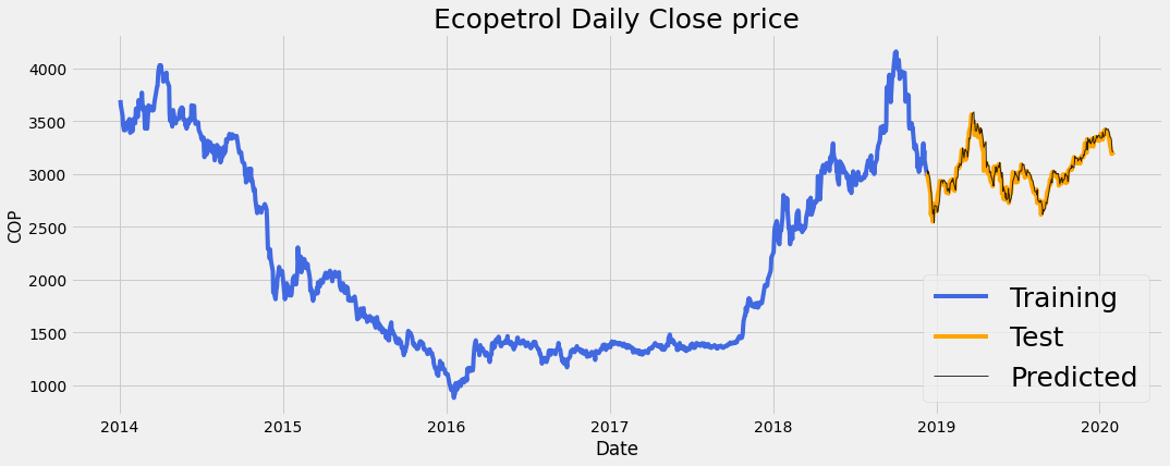
Let’s do some predictions and plot them:

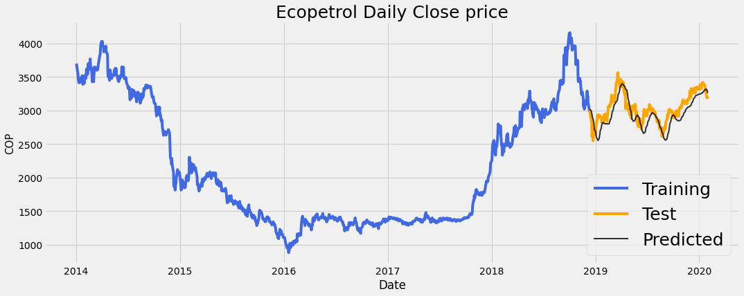
As you can see, the black line follow correctly the price movements, however there are some gaps between predicted and true movements. The performance can certainly be improve by further tuning the model

 

Next Day Prediction

Let’s predict the next day close price. Remember that the model haven’t been trained with this new date:

# Real Close Price vs. Prediction: 

Real:  3140.0
Prediction: 3217.45
Difference: 2.47%

 

Model 2

With the purpose of increase the fit and get better predictions, we will tune up the parameters:

model = Sequential()
model.add(LSTM(50, return_sequences=True, input_shape= (X_train.shape[1], X_train.shape[2])))
model.add(LSTM(50, return_sequences= False))
model.add(Dense(25))
model.add(Dense(1))

Now, plotting the test and new predicted values, we get:

The prediction fitted quite well the actual stock movements, and the MSE it’s lower than the previous model: ~0.00039147.

 

Next Day Prediction

Let’s predict the next day close price:

# Real Close Price vs. Prediction: 

Real:  3140.0
Prediction: 3159.95
Difference: 0.64%

Really close!!