K-means Clustering

Click Here to see Code

Project description: The goal of this project is to divide stocks into groups with “similar characteristics” using K-means Clustering Method. This approach can help us in portfolio construction to ensure we choose a universe of stocks with sufficient diversification between them.

 

Colecting Data

First, we need to colect stock data. To do so, we will run the script below to get the current tickers from S&P 500 Index, a stock market index that measures the stock performance of 500 large companies listed on stock exchanges in the United States.

sp500_wiki = 'https://en.wikipedia.org/wiki/List_of_S%26P_500_companies'

sp = pd.read_html(sp500_wiki)
sp = sp[0]['Symbol'].tolist()

sp500_stocks = []
for stock in sp:
    try:
        close_prices = web.DataReader(stock,'yahoo','01/01/2019')['Adj Close']
        close_prices = pd.DataFrame(close_prices)
        close_prices.columns = [stock]
        sp500_stocks.append(close_prices)
    except:
        pass
    df = pd.concat(sp500_stocks,axis=1)

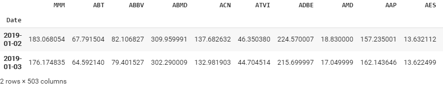
Once stock data is into a Pandas dataframe, we are ready to start the K-Means investigation.

 

Selecting the number of Clusters

How many clusters do we actually need? Rather than make some arbitrary decision we can use an Elbow Curve, often used to truncate the number of parameters in data-driven models. This method shows us the relationship between the number of clusters and the Sum of Squared Errors (SSE) resulting from using that number of clusters.

Plot the curve.

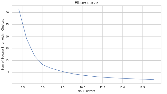
You’ll notice once the number of clusters reaches 5, the reduction in the SSE begins to slow down for each increase in cluster number. So, for this exercise we will be using 5 clusters.

 

Outliers

Regulary, when clustering data we have to deal with outliers. An outlier is an observation point that is distant from other observations.

There’s a empirical rule called “3σ approach” that states almost all data lies within 3 standard deviations of the mean for a normal distribution. In fact, this rule states that within three standard deviations is 99.7% of the data.

---

Before continue, as an example we are going to identify outliers from Apple’s stock returns using the 3σ approach

Firs, calculate the rolling mean and standard deviation. We will use a monthly window.

df2 = pd.DataFrame(web.DataReader('AAPL','yahoo','01/01/2017')['Adj Close'])

window = 21

df2['daily_ret'] = df2.pct_change()

df_rolling = df2[['daily_ret']].rolling(window=window).agg(['mean', 'std'])

Output:

Date	Adj Close	daily_ret	mean w=21	std w=21
2020-04-13	273.250000	0.019628	0.006123	0.056867
2020-04-14	287.049988	0.050503	0.002823	0.051718

 

3σ Condition:

The condition for a given observation x to be qualified as an outlier is x > μ + 3σ or x < μ - 3σ.

Plot the results:

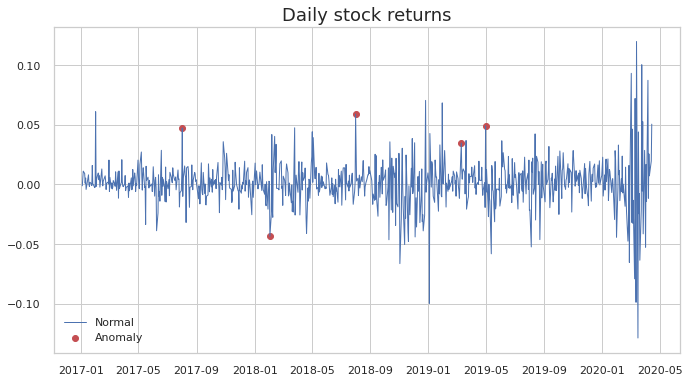
You’ll notice that when there are two large returns near one each other, the algorithm identifies the first one as an outlier and the second one as a regular observation. This might be due to the fact that the first outlier enters the rolling window (21 days) and affects the moving average/standard deviation.

---

 

Detecting Outliers: scipy.stats.zscore

The intuition behind Z-score is to describe any data point by finding their relationship with the Standard Deviation and Mean of the group of data points. Z-score is finding the distribution of data where mean is 0 and standard deviation is 1 i.e. normal distribution.

Zscore function, compute the z score of each value in the sample, relative to the sample mean and standard deviation.

Z-score Formula:

Where:

μ = Mean

σ = Standard Deviation

 

In our example, we calculate the Z-score for each observation, and re-scale and center the data looking for data points which are too far from zero. These data points which are way too far from zero will be treated as the outliers.

z = np.abs(stats.zscore(ret))
print(z)

[[0.65817816 0.72402003]
 [0.52325598 0.84873124]
 [0.112058   0.72101935]
 ...
 [0.18318992 0.39605373]
 [0.91313389 0.58136614]
 [0.91858052 0.72495043]]

Before removing outliers:

# Original dataframe
ret.shape

(503, 2)

After removing outliers:

# Modified Dataframe
ret_outliers.shape

(496, 2)

Plotting k-means clustering:

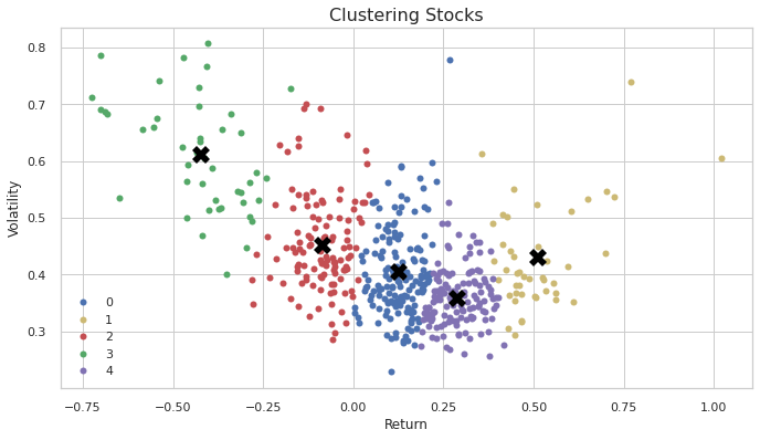
The black “X” marks are the centroids for each cluster

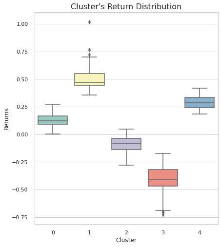
Finanlly, describe Cluster’s Return